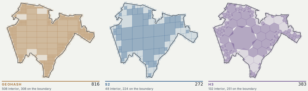
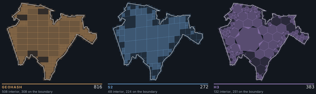
Background#
Every spatial index answers the same question: how do you flatten a 2-D surface into keys a B-tree can scan?
We were about to re-index every delivery zone in our logistics system, and the choice was going to be load-bearing for years. So I read what was out there, and found the same three paragraphs repeated everywhere:
Geohash interleaves the bits of latitude and longitude and base32-encodes them, so containment is string-prefix matching and it works in any database with no dependency at all.
S2 projects the sphere onto a cube and runs a Hilbert curve over each face, giving int64 cell IDs with exact parent-child containment.
H3 tiles an icosahedron with hexagons, so all six neighbours sit equidistant from the centre. But hexagons cannot nest, so its hierarchy is only approximate.
Those three sentences are where every comparison stops. Nobody says what any of it costs. So I measured it, and about half of what I expected turned out to be wrong.
Fixing accuracy instead of levels#
The first problem is that the obvious experiment is meaningless. “S2 level 14 versus H3 resolution 9” compares nothing, because the cells are not the same size. Whichever scheme happens to get smaller cells wins on accuracy and loses on count, and you learn nothing about the scheme.
So I inverted it. Fix accuracy, measure cost. Every scheme is tuned until its covering overshoots the true polygon by no more than a fixed excess-area budget, and then I count what it took to get there. That single choice is what makes the rest of the numbers mean anything.
There is a second trap, and I walked straight into it before catching myself. S2 returns mixed-level coverings by default: one coarse cell swallows the interior while only the boundary subdivides. H3 and geohash are normally used at a single resolution. Compare those directly and S2 wins by 10x, but you have measured adaptivity, not tiling.
So every scheme runs in two modes. Uniform pins every cell to one level, which isolates the tiling shape. Compacted lets coarse cells fill the interior and fine ones handle the edge. Both get reported.
The zones are twelve OpenStreetMap administrative boundaries across Delhi, Bengaluru and Gurugram, 4.2 to 59.8 km², eleven of them concave. Convex test polygons flatter every scheme equally and hide exactly the differences worth finding. Against those, 1.2M synthetic partner locations drawn from Pareto-weighted hotspots rather than uniformly, because uniform points understate the p99 by up to two thirds.
What a covering costs#
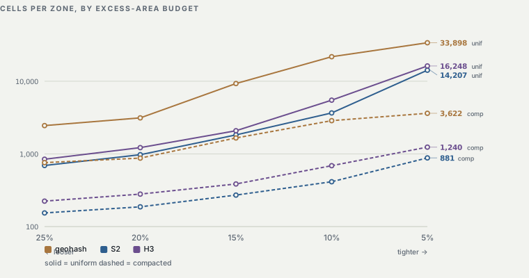
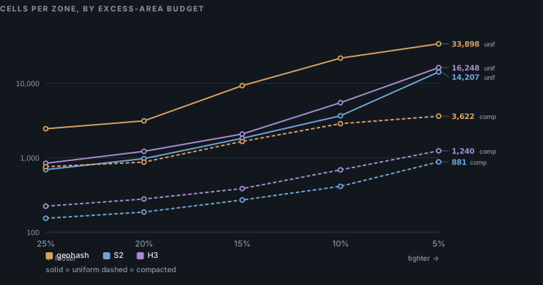
Held to a single level at matched accuracy, H3 needs the fewest cells, about 19% under S2 and half of geohash. Hexagons really do fit organic boundaries better than rectangles.
Allowed to mix levels, the order flips and S2 wins. Its exact quadtree compacts 7.7x, against 5.4x for H3 and 4.3x for geohash. So the honest answer to “which is cheapest” is: depends entirely on whether your workload can use a mixed-level covering.
The flat runs in those curves are real, and they are a cost nobody mentions. Level granularity means a budget landing between two levels pays the finer one’s full price for none of the credit. Geohash suffers worst, because its precision steps 32x in area: tightening from a 25% budget to 10% takes it from 2,457 cells to 21,767.
What H3’s approximate hierarchy actually costs#
This is the part I could not find measured anywhere. Everyone repeats that H3 parent-child containment is inexact, because hexagons cannot be subdivided into hexagons. H3 uses aperture-7 subdivision, so children are rotated slightly and spill across the parent’s edge. Nobody says how much.
So I took 100,000 resolution-9 cells, walked each to its resolution-8 parent, and clipped the child against the parent to get the exact overlap. Every scheme went through the same code, so S2’s and geohash’s zero is measured rather than assumed.
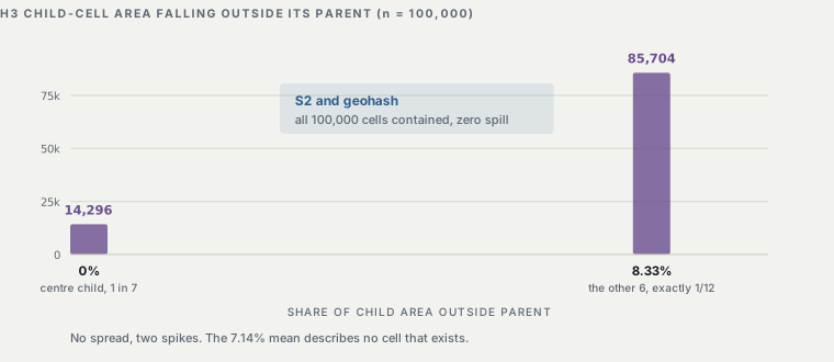
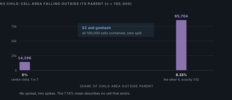
It is not a distribution. It is two spikes.
One child in seven, the centre one, is fully contained. The other six each spill exactly 1/12 of their own area, to four significant figures, every time. The 7.14% mean you would get by averaging describes no cell that exists.
That is a satisfying number, but it is geometry. The question that matters is what it does to a query.
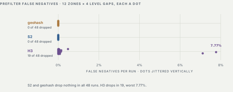
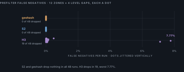
Used as a coarse-to-fine prefilter, that spill drops real matches. Cover the zone at a coarse level, keep only points whose fine cell’s ancestor is in that covering, and count what disappears. S2 and geohash drop nothing, in all 48 runs. Not almost nothing. Zero.
H3 drops matches in 19 of 48. Usually a few hundredths of a percent. Once, 7.77%.
That is a tail risk, not a rate, and the distinction matters more than the average. A dispatch system that loses one partner in thirteen, silently, with no error and no log line, is a completely different kind of problem from one that loses one in five thousand. You cannot budget for it, because it depends on how your zones happen to sit against the cell grid.
The same property breaks compaction outright. H3 ships CompactCells to merge seven children into their parent, and it is the obvious optimisation. But a parent hexagon is not the union of its children, so merging leaves 2.33% of the zone uncovered. The equivalent merge is free for S2 and geohash, whose children tile their parents exactly.
If you are using H3 resolutions as a hierarchy rather than as a flat tiling, you need a boundary-buffer pass, and that pass costs more than the hierarchy saved.
Query latency, and when it stops mattering#
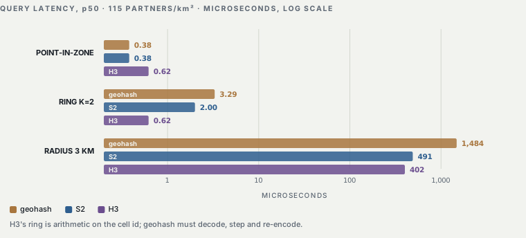
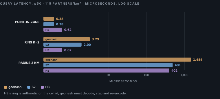
H3 wins the neighbour-driven work by 5.3x on ring traversal. Its ring is arithmetic on the cell ID, while geohash has to decode, step and re-encode, because adjacent cells can have prefixes that diverge at character two. This is the widest margin in the benchmark.
Point-in-zone is a wash. All three answer in well under a microsecond, and the ordering is inside the noise, because the work is one hash lookup and one point-in-polygon test regardless of scheme. If that is your only workload, pick on other grounds.
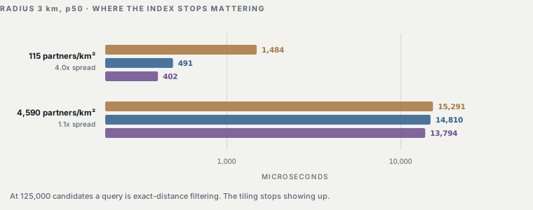
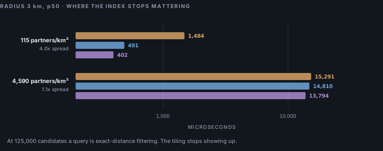
And then there is the result I did not expect, which is that past a few thousand partners per km², none of it matters.
A 3 km radius query at that density returns around 125,000 candidates. Every scheme then spends its time on exact-distance filtering, and the 3.7x spread between them collapses to 1.1x. The index choice has stopped being the thing that decides your latency. Effort belongs in capping or paginating candidates instead.
Footprint, where I had the assumption backwards#
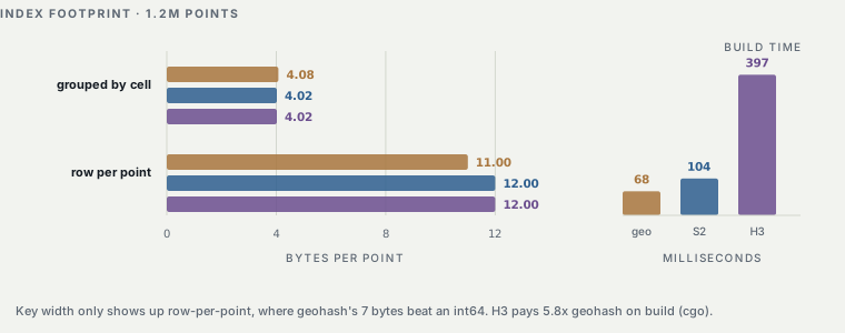
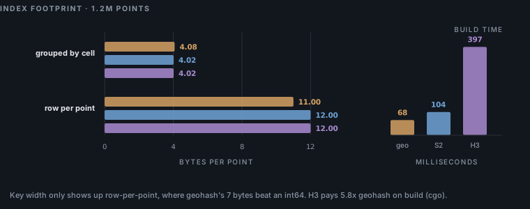
I went in expecting geohash’s variable-length string keys to cost real money at scale. They do not, twice over.
First, the layout decides whether key width matters at all. Grouped by cell, with one key and a posting list underneath, 370 points share each key and it amortises to nothing: 4.02 bytes per point against geohash’s 4.08. Key width only shows up in the row-per-point layout a B-tree actually uses, with the key repeated on every row.
Second, even there, geohash is the cheapest. At the precision that matches these cell sizes its key is 7 bytes, which is smaller than an int64. “Strings cost more than integers” only becomes true from precision 9 upward.
The real cost is somewhere I was not looking. H3 is 5.8x slower to build than geohash and 3.8x slower than S2 over 1.2M encodes. That is the cgo boundary, crossed once per point.
What I’d use where#
There is no winner, which is the honest and slightly boring conclusion.
| Workload | Pick | Why |
|---|---|---|
| Which zone contains this point? | any | all sub-microsecond; choose on other grounds |
| Partners within 3 km, sparse | H3 | fewest cells uniform, fastest radius and ring |
| Anything walking the hierarchy | S2 | exact containment; H3 drops matches, up to 7.77% |
| Compacting a covering | S2 or geohash | H3 compaction leaves 2.33% of the zone uncovered |
| No dependency allowed | geohash | prefix match anywhere; costs ~2x cells and 5.3x ring latency |
We ended up running both: S2 for zone containment and anything hierarchical, H3 for radius and aggregation, with a thin translation layer between. Two indexes over the same points cost 9.2 MB instead of 4.6 MB, which turned out to be the cheapest line item in the whole decision.
Where this benchmark is weak#
- Twelve polygons is a small sample. The concave zones drove most of the variance, and a different notch shape could move the H3/S2 gap by several points either way.
- Only one zone is from Gurugram. OSM maps few administrative boundaries there in this size range, so the set is effectively Delhi and Bengaluru.
- Synthetic points. Clustered, but from a hand-set hotspot model rather than one fitted to real order data. Real partner movement is correlated in time and mine is not, which likely flatters every scheme’s cache behaviour.
- Geohash’s radius number is confounded. Its 32x precision steps mean it cannot land near the 0.1 km² cell target and indexes 4.8x finer, so it walks more cells to fill the same disk.
- Single machine, single process. None of this captures a sharded covering table, which is where geohash’s string keys might claw something back.
- H3’s pentagons are untested. All twelve zones sit far from the twelve icosahedron vertices. If your service area includes one, budget time for it.
The harness, the zone set and the raw results are on GitHub. If you re-run it on your own zones I would be glad to see numbers that contradict these.